SuGaR: Surface-Aligned Gaussian Splatting for Efficient 3D Mesh Reconstruction and High-Quality Mesh Rendering

This is my notes on the paper SuGaR: Surface-Aligned Gaussian Splatting for Efficient 3D Mesh Reconstruction and High-Quality Mesh Rendering. For the sake of brevity, I’ve used some lines verbatim from the paper. I haven’t gottent to adding the references properly. Do excuse me for that!

Table of Contents

• Introduction
• Aligning Gaussians with the Surface
  • Part 1. Ideal Density
  • Part 2. Derive Target SDF
  • Part 3. Regularization Terms
• Mesh Extraction
  • Part 1. Sample Points using Depth Maps
  • Part 2. Identify Points on a Level Set
  • Part 3. Apply Poisson Reconstruction to Extract the Mesh
• Binding New Gaussians for Joint Refinement
• My Takeaways
• Discussion
  • Why Do We Want a Mesh
  • When Does Surface Reconstruction Struggle

---

Introduction

The goal of SuGaR is to facilitate fast and high-quality mesh extraction from 3DGS.

Meshes are currently the de facto representation used in computer graphics. While 3D Gaussian Splatting provides an explicit 3D point cloud, they’ve very hard to work with in practice. So it is desirable to represent the 3DGS scene as a mesh.

But there’s a catch! The Gaussians after Gaussian Splatting are unstructured, making it very challenging to extract a mesh from them. SuGaR presents three contributions to address this:

1. Introduces a regularization term that encourages the Gaussians to align well with the surface of the scene
2. Uses Poisson reconstruction to extract a mesh from the now well-aligned Gaussians
3. Adds an optional refinement strategy that binds and jointly optimizes the mesh and a set of 3D Gaussians

I’ll go over each of these 3 points in detail. In the end, I have included my takeaways from this paper.

Aligning Gaussians with the Surface

Part 1. Ideal Density

The density function \(d(p)\) represents the contribution of each Gaussian at any point \(p\) in space.

\[d(p) = \sum_{g} \alpha_g \exp \left( -\frac{1}{2} (p - \mu_g)^T \Sigma_g^{-1} (p - \mu_g) \right)\]

The paper formulates an ideal density function for well-aligned gaussians. It presents three properties that make a gaussian well-aligned. They are:

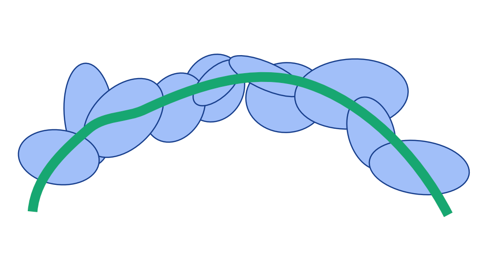
1. The Gaussians should have limited overlap with their neighbors. This encourages the Gaussians to be well-spread. This means that for any point \(p\) near the surface of the scene, the Gaussian that is closest to $p$ will contribute the most to the density function. Hence, the authors rewrite the density function focusing on the closest Gaussian \(g^*\). They also introduce a formula for finding the closest Gaussian to point \(p\).

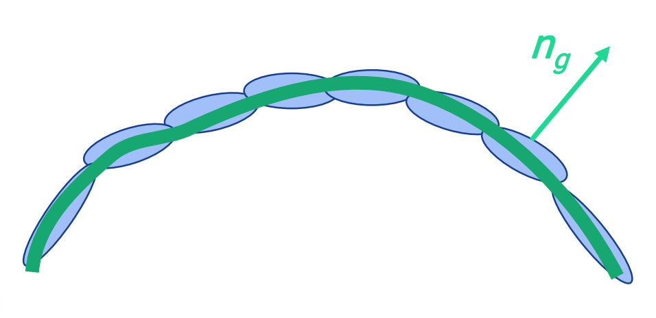
2. The Gaussians should be as flat as possible. This ensures the Gaussians are shaped more like disks aligned with the surface rather than spheres. Specifically, the scaling factor corresponding to the surface normal should be close to zero.

3. Gaussians should be either opaque or fully transparent. To represent the true surface of the scene, semi-transparent gaussians are avoided. Also, the transparent gaussians can be dropped for rendering. This means that we want \(\alpha_g = 1\) for any Gaussian \(g\).

In this ideal case, the density function becomes:

\[d(p) \approx \exp \left( -\frac{1}{2s_g^2} \langle p - \mu_g^*, n_g^* \rangle^2 \right)\]

Part 2. Derive Target SDF

Now, the authors derive an ideal SDF \(f(p)\) from this density function \(d(p)\): \(f(p) = \pm s_g^* \sqrt{-2 \log(d(p))}\) Using the SDF is more intuitive than the density function for aligning the gaussians, both in terms of distance and normals.

Part 3. Regularization Terms

Finally, they introduce the regularization term \(R\) to minimize the difference between the actual SDF of the Gaussians and the ideal SDF \(f(p)\):

\[R = \frac{1}{|P|} \sum_{p \in P} |f̂(p) - f(p)|\]

There’s two points to note here:

1. The paper uses depth maps to efficiently compute \(\hat{f}(p)\). For a sampled point \(p\), the depth map gives the distance of the surface from the camera, and the 3D position of \(p\) gives its own depth/distance. The difference of these two gives the estimated SDF.

2. Instead of just picking random points, the points are sampled according to a Gaussian distribution. This is because points near the Gaussians are more likely to be on the surface of the scene. I personally find this consideration particularly interesting: sampling Gaussians on Gaussians

The authors also introduce another regularization term, \(R_{Norm}\), to align the normals of the estimated and ideal SDFs 🎯

Mesh Extraction

Part 1. Sample Points using Depth Maps

Here, the authors are trying to sample points that are likely close to the surface.

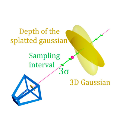
They start by randomly sampling pixels from the depth maps. This depth value gives the distance to the nearest surface from the camera along a ray. However, the depth maps are approximations. To refine, they sample additional points along this ray. Specifically, they describe sampling points \(p + t_i v\) along the ray, within 3 standard deviations.

The authors then compute the density value \(d(p)\) for each of the sampled points. In the paper, the surface is defined as the level set where \(d(p)\) equals a threshold \(\lambda\).

Part 2. Identify Points on a Level Set

To find the exact point where \(d(p) = \lambda\), linear interpolation is used. This is rather trivial. Say we find two points, one where the density value is less than \(\lambda\) and one where the density value is more than \(\lambda\). Then, we can use linear interpolation to find the point, in between these two points, where the density value equals \(\lambda\).

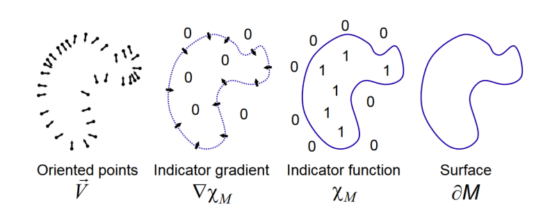
Once we have the points on the level set, we also compute the normals of these points, using the normalized analytical gradient of their density function.

Part 3. Apply Poisson Reconstruction to Extract the Mesh

Now we have a set of 3D points on the surface and their normals. This is the perfect setup to use Poisson Reconstruction to generate a triangle mesh.

The authors illustrate how this approach is better than using Marching Cubes. Marching Cubes can work well with a few thousand Gaussians. However, in practice, a scene can have millions of Gaussians. For the explicit representations we have, Poisson Reconstruction is more suited than Marching Clouds for a smooth mesh output.

To decrease the resolution of the meshes, the authors also employ mesh simplification using quadric error metrics.

Binding New Gaussians for Joint Refinement

Now that we have an initial mesh, the authors propose to bind new Gaussians to the surface of this mesh, then jointly optimize the mesh and the bound Gaussians.

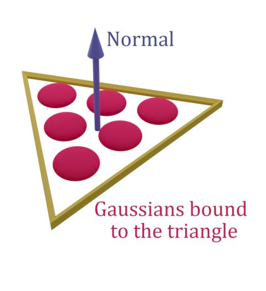
On each triangle, \(n\) new 3D Gaussians are instantiated. The parameterization here is similar to GaMeS (I’m just using this point to explain the intuition). The implementation details used here, to keep the gaussians flat and aligned to the surface, are:

• Use barycentric coordinates for the means.
• Only optimize a 2D rotation in the triangle’s plane. This is encoded with a complex number \(x +iy\), rather than the previous quaternion for 3D rotation.
• Only optimize 2 scaling factors instead of 3. The scaling along to normal is set to be very small.
• Opacity and color parameters remain similar to the original paper.

According to the authors, this helps with reconstructing fine-details, thus increasing render quality. The mesh extracted after the first optimization stage serves as an excellent initialization for positioning Gaussians when starting the refinement phase.

During joint refinement, the authors also regularize the normal on the mesh’s faces to promote smoother surfaces.

My Takeaways

• Even with mesh refinements, I noticed SuGaR had lower rendering performance than both vanilla 3DGS and Mip-NeRF360. My understanding is that SuGaR struggles with small fuzzy details, since it is trying to reconstruct the scene as a surface entirely. (more on this in the disucussions here)

• To me, sampling and identifying points on the level set for mesh extraction seemed similar to ray marching in NeRF. And so I assumed that it would be time-consuming. However, here its actually faster because the search space is much smaller. The use of depth maps provides a good starting point. And afterwards, instead of all the points, only a range of points are sampled. Additionally, SuGaR uses linear interpolation between two points instead of evaluating the entire ray. Thus the process becomes more targeted and efficient than traditional NeRF ray marching.

• For mesh extraction, two Poisson reconstructions are applied: one for foreground points, and one for background points. I find this idea similar to the coarse and fine networks used in NeRF. The use-case here is of course different. Nonetheless, I think this allows for a more robust reconstruction of the main objects. The authors use bounding boxes to separate foreground points from background, and I’m curious whether segmentation masks can offer better results.

• I personally enjoyed reading about SuGaR more, and writing about GaMeS more. I think SuGaR is a very comprehensive paper, and it helped me visualize and grasp many of the surrounding ideas, like marching cubes and poisson reconstruction. The hybrid representations in the optional refinement stage leads to more sophisticated approaches, like GaMes, that can allow for real-time deformations.

Discussion

I thought I’d add this section to briefly discuss some key concepts

Why Do We Want a Mesh

Structure and Control.

Let’s elaborate. Gaussian Splatting can be thought of as a new way of reconstructing point clouds, without relying on the hard geometry. But, as a tradeoff, we don’t get any surfaces. GS also introduces an issue with deterministic reconstruction of a scene, but we’ll talk about that more in dynamic gaussians. Here though, even for a single scene, incorporating the output of vanilla 3DGS into traditional graphics pipelines is challenging.

This goes back to what we saw in GaMeS that the reason we need a mesh is to be able to deform it for animation. Meshes offer an well-structured representation of an object’s geometry. For scenarios that require interactivity and manipulation, such as gaming or film animations, having a mesh is beneficial (the book Physically Based Rendering: From Theory To Implementation helped me see how PBR has been used in films with some stunning visual examples). In character animation, meshes are essential for rigging. Meshes are also convenient for physical simulations, such as collisions and deformations.

When Does Surface Reconstruction Struggle

I’m going to try and look at this from my understanding of the fundamentals.

Let us start with the physically-correct way of rendering. My understanding is that physically-correct rendering means the system simulates how light behaves in the real world. And, to add to this, according to the pbrt book: ray tracing is conceptually a simple algorithm; it is based on following the path of a ray of light through a scene as it interacts with and bounces off objects in an environment. So, in physically-correct rendering, we have to consider properties such as refractions, light scattering at surfaces, indirect light transport, ray propogation and more.

Surface meshes, on the other hand, are designed for computational efficiency, not accuracy in light simulation. Here, we assume that objects are composed of hard surfaces. By reconstructing our Gaussians to surfaces entirely, we lose their inherent volumetric properties. So it becomes much harder to recover volumetric effects (fire/smoke), or fuzzy materials (hair/grass). With just surfaces, its much difficult to model the physical properties of light. For example, in this image, I believe we would not be able to model the interaction of light underneath the the snow if we just considered the surface representation.

this concludes my notes on the paper SuGaR: Surface-Aligned Gaussian Splatting for Efficient 3D Mesh Reconstruction and High-Quality Mesh Rendering.