PhysGaussian: Physics-Integrated 3D Gaussians for Generative Dynamics
This is my notes on the paper PhysGaussian: Physics-Integrated 3D Gaussians for Generative Dynamics. For the sake of brevity, I’ve used some lines verbatim from the paper. Also, I haven’t gottent to adding the references properly. Do excuse me for that!
Table of Contents
- Introduction
- How It Works
- Theory
- Implementation Details
- Optimizations
- Discussion
Introduction
PhysGaussian enables physically-grounded, novel movement synthesis by linking Gaussians in 3DGS with an underlying Material Point Method (MPM) framework rooted in Continuum Mechanics (CM). Initially, I found the concept rather intimidating. But once I broke it down, it became surprisingly intuitive. What I found elegant about PhysGaussian is that, although it achieves dynamic behavior, the Gaussians themselves don’t need to explicitly model this dynamism. Instead, the MPM framework drives the physics, transferring changes to the Gaussians at each time step. Notably, the paper:
-
Introduces a way to map Gaussians to the MPM framework, enabling continuum mechanics-based 3D Gaussian kinematics
-
This unified representation allows for a seamless simulation-rendering pipeline, i.e it does not need intermediary representations such as explicit meshes
-
Compared to the other approaches in the literature, PhysGaussian achieves more physically grounded results. Particularly, the optimizations align closely with real-world object physics
Here, I’ll focus on how PhysGaussian models physics-integrated Gaussians over time, rather than diving into MPM and Continuum Mechanics. I belive the main focus of the paper is really on integrating these concepts rather than on the details of the frameworks themselves.
The following chapters are organized in the order that I worked through the paper. First, we outline the overall approach, then we dive deep into the cores ideas, next we understand some of the implementation details to get a better grasp, and finally conclude with the optimizations that help refine the results.
How It Works
In essence, each Gaussian kernel acts as a particle in the object. MPM handles the physics between these particles, simulating interactions and deformations. As the simulation progresses, Gaussians update their physical and visual properties, and these updates are rendered to show the object’s behavior in real-time.
Here’s a quick summary of how it all ties together:
-
Images + SfM → 3D Gaussian Representation
-
Setting up Physics Properties for the Gaussians: The Gaussians are assigned physical properties based on the 3D representation. This lets each Gaussian kernel act as a particle in the MPM simulation.
-
MPM Simulation Steps: In each time step, the mass and momentum from the particles are transferred to the grid. The grid is then used to handle physics simulations, such as collisions, internal forces and more. The resulting calculations update the grid. The updates (positions, velocity, deformation) are then transferred back to the particles.
-
Update of Gaussians: Each Gaussian’s properties are updated in response to the physical interactions calculated by the MPM. For example, if a Gaussian kernel collides with another object, its velocity, position, and shape will adjust accordingly, as directed by the MPM physics.
-
Visual Rendering: With the updated properties, each Gaussian kernel is rendered in its new position and shape, resulting in a visually accurate representation of the physical simulation. This means we see the visual effects of physical phenomena like collisions, stretching, and compression directly in the Gaussian render, as they evolve in time with the simulation.
So, as the MPM simulation computes and updates the state of each Gaussian in response to forces, collisions, and interactions, the rendered Gaussians reflect these changes. This is what makes it seamless - it unifies simulation and rendering, so the visuals are always in sync with the underlying physics!
Theory
3.1. Continuum Mechanics & Material Point Method
CM provides the theoretical foundation and MPM is the framework that implements/simulates that behavior. Using MPM, the paper models how the Gaussians’ properties change over time, effectively simulating physical dynamics. Let’s talk about some of the key ideas here.
3.1.1. Key Ideas from Continuum Mechanics
Deformation Map: In continuum mechanics, deformation is described through the deformation map \(\varphi(X, t)\), which moves each material point from an original position \(X\) to a deformed position \(x = \varphi(X, t)\) over time \(t\). This is the zero-order information.
Deformation Gradient: The deformation gradient \(F\) provides information about how each local material region stretches, rotates, or shears during deformation. It is the first-order deriavative of the deformation map.
Conservation Laws:
-
Mass Conservation: Mass remains constant within any region of the material. Mathematically:
\[\int_{B_{\epsilon}^t} \rho(x, t) \equiv \int_{B_{\epsilon}^0} \rho(\phi^{-1}(x, t), 0)\]where \(B_0\) is a region in the initial (undeformed) configuration and \(B_t\) is the corresponding region in the deformed state.
-
Momentum Conservation: The rate of change of momentum in the material must balance with the forces (internal and external). Mathematically:
\[\rho(x, t) \, \dot{v}(x, t) = \nabla \cdot \sigma(x, t) + f_{\text{ext}}\]where \(\sigma(x, t)\) is the Cauchy stress tensor representing internal forces, \(\rho(x, t)\) is the density, \(v(x, t)\) is the velocity, and \(f_{\text{ext}}\) is an external force per unit volume.
3.1.2. Key Ideas from Material Point Method
Discrete Particles and Grids: MPM discretizes the continuum by combining particles (Lagrangian) and grids (Eulerian). Each particle represents a small material region and tracks position, velocity, and deformation properties. These particles interact with a grid to handle momentum and collision. This allows MPM to simulate how the entire material body deforms, even when it undergoes complex behaviors like collision or fracture.
MPM Update Process Overview: For each time step:
-
The particle’s mass and momentum (mass × velocity) are transferred to nearby grid nodes, weighted by distance.
-
Now, the system calculates forces at each grid node based on internal stress \(\sigma\) and external forces, such as gravity \(g\). These forces are then used to update grid velocities. This is done using forward Euler integration.
-
After updating the grid, MPM transfers the new velocities and positions back to the particles.
-
The deformation gradient \(F\) is also updated. This also contains specific mappings for plasticity and stress.
3.2. Physics-Integrated 3D Gaussians
I’m going to cover two main ideas here. First, how physics properties are integrated into Gaussians to model them as particles. Second, how the updated particle properties from MPM are transferred back to the Gaussians.
3.2.1. Setting up Physics Properties for the Gaussians
- Assigning Mass: The mass \(m_p\) for each Gaussian kernel is set based on:
- Volume: Each Gaussian has an associated volume \(V_p^0\), which is approximated based on its initial covariance.
- Density: The user specifies a density \(\rho_p\) for each Gaussian, based on assumptions about the material (e.g., density of rubber, metal, or sand).
- The mass for each Gaussian is then calculated as: \(m_p = \rho_p V_p^0\)
- Initializing Velocity: The initial velocity \(v_p\) of each Gaussian kernel is set according to the initial state of the object. This could mean:
- Setting all initial velocities to zero (for an object starting at rest).
- Adding an initial motion if specified (e.g., a controlled movement or an external force acting on the object).
3.2.2. Applying the Deformation to Gaussian Kernels
This is where we update each Gaussian kernel’s properties to reflect the simulation results.
-
First, let’s define each Gaussian kernel in the original material configuration: \(G_p(X) = e^{-\frac{1}{2} (X - X_p)^T A_p^{-1} (X - X_p)}\)
Here \(X_p\) and \(A_p\) give the Gaussian’s center and shape before deformation.
-
Now we apply the deformation to each kernel using the deformation gradient \(F_p\). When the deformation map \(\varphi(X, t)\) is applied, the Gaussian \(G_p\) should ideally remain Gaussian in the deformed space. However, directly applying the map may distort it in ways that don’t preserve its Gaussian form. To maintain the Gaussian shape, the paper assumes a local affine transformation: \(\tilde{\varphi}_p(X, t) = x_p + F_p (X - X_p)\)
- Next, we want to understand how this affine transformation changes the position and shape of the Gaussian.
- Center Position \(x_p(t)\): The center of the Gaussian in the deformed space is simply \(x_p(t) = \varphi(X_p, t)\). This places the center where it should be in the deformed material.
- Covariance Matrix \(a_p(t)\): This makes sure the Gaussian stretches or rotates according to the deformation. In the deformed space, this becomes: \(a_p(t) = F_p A_p F_p^T\)
- Finally, we render the updated Gaussian with its new center and shape: \(G_p(x, t) = e^{-\frac{1}{2} (x - x_p)^T (F_p A_p F_p^T)^{-1} (x - x_p)}\)
The Gaussian opacity \(\sigma_p\) and spherical harmonics remain constant in this implementation. However, we do rotate the view direction for the spherical harmonics to maintain consistency. This is discussed in the next section.
3.3. Evolving Orientations of Spherical Harmonics
When objects deform or rotate, the orientation of the Gaussian’s SH must adjust accordingly so that the rendered object looks realistic from different angles. Instead of recalculating new spherical harmonics bases for each rotation, the authors apply a rotation to the view direction to keep the color consistent. I think the figure below makes this really intuitive to understand.
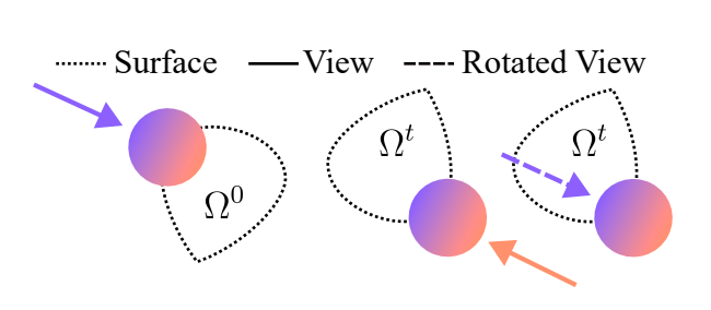
Specifically, they use the polar decomposition of the deformation gradient \(F_p\) to separate rotation \(R_p\) and scaling/stretching \(S_p\). \(F_p = R_p S_p\)
Now, we can use \(R_p\) to update the spherical harmonics bases, which depends on view direction \(d\), as: \(f_t(d) = f_0(R_p^T d)\)
Implementation Details
Q1. How do we know which objects are which Gaussians? In 3DGS, the Gaussians are placed somewhat arbitarily. Also, a single object can have multiple Gaussians.
We actually define this ourselves here. Gaussians that represent different parts of an object are grouped into regions based on user input. These regions correspond to specific parts of the scene that the user intends to simulate dynamically (e.g., an area that will bend or fracture).
Q2. How do the objects know how to behave? How do we infer the properties from their SfM input?
This is also done manually. Here, we additionally assign material properties to each region. For instance, for a part of the scene with sand, we would use the Drucker-Prager model for granular behavior.
As for the second part of the question, that’s not within the scope of this paper. It is mentioned in the discussions, and I belive is another interesting research direction to explore.
Q3. How do the Gaussians know how to deform? Like, do we specify that a force is coming from a certain direction?
Well, yes! Alongside the material properties, we also selectively modify the velocities of specific particles (as discussed here) to induce controlled movement or forces in the simulation. The remaining particles then follow natural motion pattern governed by the established MPM framework.
Q4. What is the purpose of the Simulation Cube?
We manually define a specific region of the scene for the simulation. This is where the drama unfolds. This cube, scaled to an edge length of 2 units, acts as a boundary for the simulation. Inside this cuboid simulation domain, we create a dense 3D grid. This grid represents the simulation space.
Optimizations
Here, I’d like to briefly discuss two particular optimization and regularization used the paper.
5.1 Internal Filling
Typically, Gaussians are distributed near the surface of an object, which creates a hollow interior. For realistic deformations, the authors generate internal particles within the object by estimating a density field from the opacities of existing Gaussians. The density field \(d(x)\) is defined as: \(d(x) = \sum_{p} \sigma_p \exp \left( -\frac{1}{2} (x - x_p)^T A_p^{-1} (x - x_p) \right)\)
Here, \(\sigma_p\) is the opacity of each Gaussian, and \(A_p\) is its covariance matrix.
The authors discretize this density field onto a 3D grid, then set an opacity threshold \(\sigma_{\text{th}}\) to define “interior” cells. Rays are cast along several axes to identify regions within this threshold. To ensure visual consistency after deformation, the interior particles inherit properties, like opacity \(\sigma_p\) and spherical harmonics \(C_p\), from nearby surface particles. Their covariances are initialized as \(\text{diag}(r_p^2, r_p^2, r_p^2)\), where \(r\) is the particle radius calculated from its volume: \(r_p = \left( \frac{3 V_p^0}{4 \pi} \right)^{1/3}\)
5.2 Anisotropy Regularizer
Under large deformations, some Gaussian kernels can become overly stretched or “skinny.” This leads to visual artifacts, creating a “plush” effect. To control this, the authors add a regularization term that limits how much a Gaussian can stretch in one direction relative to others. This prevents extreme anisotropy (one direction becoming much longer or shorter than others). Mathematically, for each Gaussian kernel, let \(S_p\) represent its scaling values. The regularizer then becomes: \(L_{\text{aniso}} = \frac{1}{|P|} \sum_{p \in P} \max\left( \frac{\max(S_p)}{\min(S_p)}, r \right) - r\)
Here, \(r\) is a user-defined threshold. Among all the regularization terms I’ve come across in 3DGS so far, this is probably my favorite one!
Discussion
Here, I am going to discuss some fundamental questions regarding PhysGaussian. For question 2 and 3, I referenced this paper: Neural Stress Fields for Reduced-order Elastoplasticity and Fracture, which is the MPM implementation used in PhysGaussian
6.1 What is the fundamental problem they are trying to solve?
At its core, this work addresses the gap between high-quality physical simulations and visually consistent rendering.
In conventional graphics workflows, physical simulations generate realistic motions and deformations, but translating these into high-quality visual representations involves multiple, often cumbersome stages. For instance, conventional approaches, i.e NeRFshop (NeRF-based) or GSDeformer (3DGS-based), rely on generating intermediary geometric representations like cage meshes, which may not align perfectly between the simulated and rendered versions of an object. This discrepancy is what PhysGaussian’s unified representation addresses.
6.2 How is the problem solved in traditional physics?
In classical physics, problems related to deformation and motion of materials are often solved using continuum mechanics. This involves solving partial differential equations that describe the properties like motion, stress, interactions of materials under forces.
Frameworks like MPM can simulate dynamics by tracking physical properties such as position, velocity, and deformation over time. MPM discretizes a physical material into particles and grids, allowing it to handle complex behaviors, e.g. large deformations, topology changes, and self-contact.
6.3 What’s wrong with the pure physics-based simulation approach?
Well, first of all, computational complexity! MPM’s versatility comes at the cost of computation burden, in terms of both long runtime and excessive memory consumption. MPM has to track a large number of state variables for the particles. Another challenge is synchronizing the high-dimensional state variables. For instance, in VR or cloud gaming, multiple users share the same simulated physical environment. Vanilla MPM computation proves to be a bottleneck here. In fact, the custom MPM implementation used in PhysGaussian uses reduced order modeling (ROM) to perform dimensionality reduction and alleviate the computation overhead.
6.4 What does 3DGS offer?
I think the explicit, structured representation in 3DGS is a key distinction. Since each Gaussian already has a physical location and extent, it intuitively leads to many of the integrations we see in the literature.
I believe this is foundational to PhysGaussian’s unified representation. In contrast, methods like NeuPhysics need to rely on separate MLPs to handle different attributes like motion, rigidity, and SDFs. Gaussians are relatively low-cost primitives that can be independently manipulated. Together, these qualities make PhysGaussian more robust than counterparts like PAC-NERF.
this concludes my notes on the paper PhysGaussian: Physics-Integrated 3D Gaussians for Generative Dynamics. thank you for reading!